Autoformer
논문: Autoformer: Decomposition Transformers with Auto-Correlation for Long-Term Series Forecasting
개요
Anomaly Transformer 깃허브에서 레포지토리의 Fork와 Star가 많아서 논문을 읽어보기로 했다.
찾아 본 영단어
Immanent: existing or operating within; inherent. 내재하는
Seamlessly: smoothly and continuously, with no apparent gaps or spaces between one part and the next. 원활하게
Seam: 이음매
요약
Abstract
- 전통적인 transformer 기반 모델은 복잡한 장기적 시간 패턴 및 효율성에 어려움이 있음
- Autoformer는 복잡한 시계열을 처리할 수 있는 능력을 향상하기 위해 시계열 분해(series decomposition)를 핵심 구성 요소로 통합
- Auto-Correlation은 부분 시계열 수준(sub-series level)에서 작동하여 의존성을 효과적으로 발견하고 표현을 집계
1 Introduction
- 장기적 미래의 복잡한 시간적 패턴을 해결하기 위해, Autoformer를 분해 아키텍처로 제시
- 내재적인 점진적 분해 능력을 갖춘 딥 예측 모델을 위해 inner decomposition block을 설계
- series level에서 의존성 발견 및 정보 집계를 위한 Auto-Correlation 메커니즘을 제안
- 이전의 self-attention 패밀리를 넘어서 동시에 계산 효율성과 정보 활용성을 개선
- Autoformer는 에너지, 교통, 경제, 날씨 및 질병을 다루는 다섯 가지 실제 응용 프로그램을 포함한 여섯 가지 벤치마크에서 장기 설정에서 38% 상대적 개선을 달성
2 Related Work
2.1 Models for Time Series Forecasting
- ARIMA과 같은 고전적인 도구부터 시작하여 다양한 모델이 시계열 예측에 사용됨
- ARIMA는 차분을 통해 비정상적인 과정을 정상적인 과정으로 변환
- 다른 방법에는 필터링 및 순환 신경망(RNNs)이 포함됨
- DeepAR 및 LSTNet과 같은 모델은 자기 회귀 기법을 RNNs 또는 CNNs와 결합하여 시간적 패턴을 포착
- attention 기반 RNNs 및 temporal convolution networks(TCN)는 각각 장거리 의존성 및 시간적 인과 관계를 탐색
- self-attention에 기반한 Transformers는 순차적 데이터에서 강력함을 보이지만 장기적인 예측에는 계산적으로 어렵움
- LogTrans, Reformer 및 Informer와 같은 최근 변형은 복잡성을 줄이려고 하지만 여전히 point-wise 의존성과 집계를 의존
- 본 논문은 시계열의 주기성을 활용하여 시계열 간 연결에 대한 Auto-Correlation 메커니즘을 소개
2.2 Decomposition of Time Series
- 시계열 분해는 데이터를 예측 가능한 패턴으로 분해함
- 역사적 분석 및 예측에 유용함
- 기존 방법은 전처리로 사용되지만 장기적인 패턴 상호작용을 놓칠 수 있음
- Autoformer는 심층 모델 내에서 분해를 통합함
- 점진적 예측을 가능하게 함
- 과거 및 예측된 데이터를 모두 고려함
3 Autoformer
시계열 예측 문제란,
길이가 $I$인 과거의 series가 주어졌을 때, 길이가 $O$인 가장 가능성 있는 미래의 series를 예측하는 것
- 표기: ${input-I-predict-O}$
- ${long-term forecasting}$: 장기적 미래, 즉 더 큰 $O$를 예측하는 것
장기 시계열 예측의 어려움
- 복잡한 시간적 패턴 처리
- 계산 효율성과 정보 활용성의 병목 현상
3.1 Decomposition Architecture
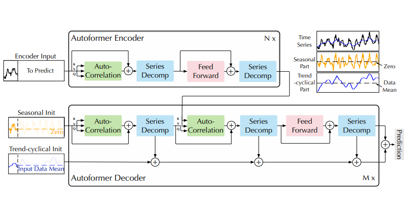
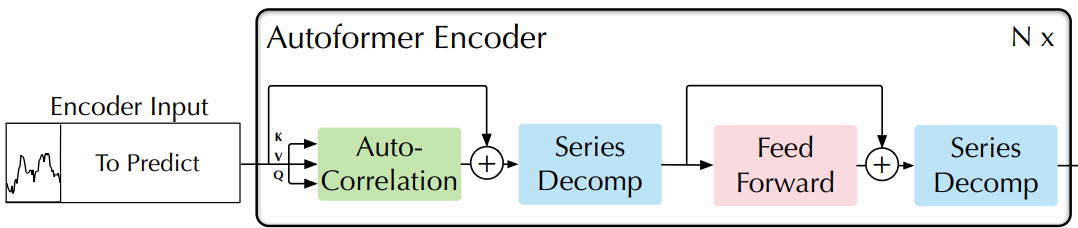
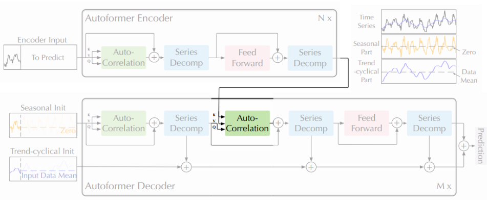
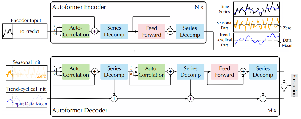 Figure 1: Autoformer architecture
- Encoder는 series decomposition blocks을 사용하여 장기적인 추세-주기 부분을 제거하고 계절 패턴 모델링에 집중
- Decoder는 숨겨진 변수에서 추출된 추세 부분을 점진적으로 누적
- Encoder에서의 과거 계절 정보는 Encoder-Decoder Auto-Correlation에 의해 활용
Series decomposition block
- 장기적인 예측에서 복잡한 시간적 패턴 처리하기 위해, series를 추세-주기 및 계절적 부분으로 분해
- 그러나 알려지지 않은 미래 데이터를 직접 분해하는 것은 비현실적
- 이를 해결하기 위해 Autoformer 내에 series decomposition block 도입
- 예측된 중간의 숨겨진 변수에서 장기적인 안정된 추세를 추출
- 모델이 생성한 중간 표현에서 데이터의 기저 장기적인 추세를 식별하고 분리
- 시간이 지나도 지속되고 단기적인 변동이나 잡음에 영향 받지 않는 패턴 식별
- 주기적인 변동을 완화하고 장기적인 추세를 강조하기 위해 이동 평균을 사용
길이-$L$ 입력 series $\mathcal{X} \in \mathbb{R}^{L×d}$
\[\begin{equation} \begin{split} & \mathcal{X}_{\text{t}} = \text{AvgPool}(\text{Padding}(\mathcal{X})) \\ & \mathcal{X}_{\text{s}} = \mathcal{X} − \mathcal{X}_{\text{t}} \end{split} \end{equation}\]- \(\mathcal{X}_{\text{s}}, \mathcal{X}_{\text{t}} ∈ \mathbb{R}^{L×d}\) : 각각 계절(seasonal) 및 추세-주기(trend-cyclica) 부분
- series의 길이를 변경하지 않기 위해 이동 평균에 대한 패딩 작업과 함께 $\text{AvgPool}(·)$을 채택
- 요약식: \(\mathcal{X}_{\text{s}}, \mathcal{X}_{\text{t}} = \text{SeriesDecomp}(\mathcal{X} )\)
Model inputs
- 인코더의 입력: 과거 $I$ 타임 스텝 $\mathcal{X}_{\text{en}} \in \mathbb{R}^{I×d}$
- 디코더의 입력: 계절 부분 \(\mathcal{X}_{\text{des}} \in \mathbb{R}^{(\frac{I}{2} +O)×d}\)과 추세-주기 부분 $\mathcal{X}_{\text{det}} \in \mathbb{R}^{(\frac{I}{2} +O)×d}$이 포함
- 각 초기화는 두 부분으로 구성
- 최근 정보를 제공하기 위해 길이가 $\frac{I}{2}$인 인코더 입력 $\mathcal{X}_{\text{en}}$의 후반부로부터 분해된 구성 요소
- 스칼라 값으로 체워진 길이 $O$의 placeholder
- \(\mathcal{X}_{\text{ens}}, \mathcal{X}_{\text{ent}} \in \mathbb{R}^{\frac{I}{2}×d}\) : 각각 $\mathcal{X}_{\text{en}}$의 계절 부분과 추세-주기 부분
- \(\mathcal{X}_{0}, \mathcal{X}_{\text{Mean}} \in \mathbb{R}^{O×d}\) : 각각 $0$과 $\mathcal{X}_{\text{en}}$의 평균으로 체워진 placeholder
Encoder
- 인코더는 계절 부분 모델링에 집중
- 인코더의 출력
- 과거의 계절 정보 포함
- 디코더가 예측 결과를 미세 조정하는 데 도움이 되는 교차 정보(cross information)으로 사용
- $N$ 개의 인코더 레이어 가정
- $l$번째의 인코더의 식: \(\mathcal{X}^{l}_{\text{en}} = \text{Encoder} ( \mathcal{X}^{l-1}_{\text{en}} )\)
- “_”: 생략되는 부분
- \(\mathcal{X}^{l}_{\text{en}} = \mathcal{S}^{l, 2}_{\text{en}}\) : $l$번째 인코더 레이어의 출력, $l \in {1, …, N}$
- \(\mathcal{X}^{0}_{\text{en}}\) : $ \mathcal{X}_{\text{en}}$의 임베딩
- $ \mathcal{S}^{l, i}_{\text{en}}$: $l$번째 레이어의 $i$번째 series decomposition block 이후의 계절 요소, $i \in {1, 2}$
Decoder
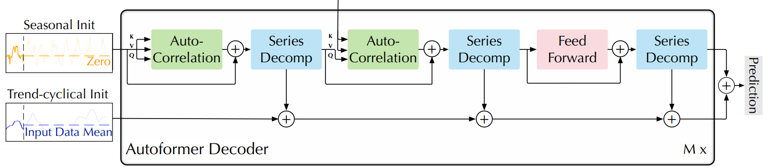
- 디코더는 두 부분으로 구성
- 추세-주기 성분을 위한 누적 구조
- 계절 성분을 위한 stacked Auto-Correlation 메커니즘
- 각 디코더 레이어는 inner Auto-Correlation 및 encoder-decoder Auto-Correlation을 포함
- inner Auto-Correlation: 예측을 미세 조정
- encoder-decoder Auto-Correlation 과거 계절 정보를 활용
- 모델은 디코더 중간 숨겨진 변수에서 잠재적인 추세를 추출
- 추세 예측을 점진적으로 미세 조정
- Auto-Correlation에서의 주기적인 의존성 발견을 위한 간섭 정보 제거
$M$ 개의 디코더 레이어 가정
인코더부터의 latent variable: $\mathcal{X}^N_{\text{en}}$
$l$번째 디코더 레이어 식: \(\mathcal{X}^l_{\text{en}} = \text{Decoder}(\mathcal{X}^{l-1}_{\text{de}}, \mathcal{X}^{N}_{\text{en}})\)
디코더 공식:
\[\begin{equation} \begin{split} \mathcal{S}^{l,1}_{\text{de}}, \mathcal{T}^{l,1}_{\text{de}} &= \text{SeriesDecomp}\left(\text{Auto-Correlation}(\mathcal{X}^{l-1}_{\text{de}}) + \mathcal{X}^{l-1}_{\text{de}}\right) \\ \mathcal{S}^{l,2}_{\text{de}}, \mathcal{T}^{l,2}_{\text{de}} &= \text{SeriesDecomp}\left(\text{Auto-Correlation}(\mathcal{S}^{l,1}_{\text{de}}, \mathcal{X}^{N}_{\text{en}}) + \mathcal{S}^{l,1}_{\text{de}}\right) \\ \mathcal{S}^{l,3}_{\text{de}}, \mathcal{T}^{l,3}_{\text{de}} &= \text{SeriesDecomp}\left(\text{FeedForward}(\mathcal{S}^{l,2}_{\text{de}}) + \mathcal{S}^{l,2}_{\text{de}}\right) \\ \mathcal{T}^{l}_{\text{de}} &= \mathcal{T}^{l-1}_{\text{de}} + \mathcal{W}_{l,1} \ast \mathcal{T}^{l,1}_{\text{de}} + \mathcal{W}_{l,2} \ast \mathcal{T}^{l,2}_{\text{de}} + \mathcal{W}_{l,3} \ast \mathcal{T}^{l,3}_{\text{de}} \end{split} \end{equation}\]- $\mathcal{X}^{l}_{\text{de}}$ : $l$번째 디코더 레이어 출력, $l \in {1, …, M}$
- \(\mathcal{X}_{\text{de}}^{0}\) : \(\mathcal{X}_{\text{des}}\)에서의 임베딩 for deep transform
- \(\mathcal{T}_{\text{de}}^0 = \mathcal{X}_{\text{det}}\) : for accumulation
- $\mathcal{S}_{\text{de}}^{l, i}$: $l$번째 레이어의 $i$번째 series decomposition block으로부터의 계절적 요소, $i \in {1,2,3}$
- $\mathcal{T}_{\text{de}}^{l, i}$: $l$번째 레이어의 $i$번째 series decomposition block으로부터의 추세-주기 요소, $i \in {1,2,3}$
- \(\mathcal{W}_{l, i}\) : projector for $i$번째 추출된 추세 \(\mathcal{T}_{\text{de}}^{l, i}\)
- 최종 예측: 두 개의 세분화된 구성 요소의 합 \(\mathcal{W}_\mathcal{S} \ast \mathcal{X}^M_{\text{de}} + \mathcal{T}^M_{\text{de}}\)
- \(\mathcal{W}_\mathcal{S}\) : 심층 변환된 계절 성분 \(\mathcal{X}^M_{\text{de}}\) 을 대상 차원으로 투영하기 위해
3.2 Auto-Correlation Mechanism
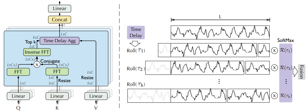 Figure 2: Auto-Correlation (left) and Time Delay Aggregation (right)
- 정보 활용을 확장하기 위해 series-wise 연결을 갖는 Auto-Correlation 메커니즘을 제안
- series autocorrelation을 계산하여 주기별 종속성을 발견
- 시간 지연 집계를 통해 유사한 sub-series를 집계
Period-based dependencies
주기의 같은 위상 위치(phase position)는 유사한 sub-processes를 제공 실제 이산시간 과정 \({\mathcal{X}_{t}}\)에 대해 다음 방정식을 통해 autocorrelation \(\mathcal{R}_{\mathcal{X}\mathcal{X}}(τ)\)을 얻을 수 있다.
\[\begin{equation} \begin{split} \mathcal{R}_{\mathcal{X}\mathcal{X}}(\tau) = \lim_{L\to\infty} \frac{1}{L} \sum_{t=1}^L \mathcal{X}_{t} \mathcal{X}_{t-\tau} \end{split} \label{eq:eq5} \end{equation}\]- $\mathcal{R}_{\mathcal{XX}}(τ)$ : \({\mathcal{X}_{\text{t}}}\) 와 그의 $\tau$ lag series \({\mathcal{X}_{t-\tau}}\) 간의 시간 지연 유사성 반영
- autocorrelation $\mathcal{R}(\tau)$ 를 추정된 주기 길이 $\tau$ 의 정규화되지 않은 신뢰도 사용
- 그런 다음, 가장 가능성 있는 $k$ 개의 주기 길이 $ \tau_1, … , \tau_k $ 를 선택
- period-based dependencies
- 추정된 주기에 의해 파생
- 해당하는 autocorrelation에 의해 가중될 수 있음
Time delay aggregation
- period-based dependencies은 추정된 기간 간의 하위 시리즈를 연결
- 선택된 시간 지연 $\tau_1, · · · , \tau_k$에 기반하여 시리즈를 롤링할 수 있는 time delay aggregation block을 제안
- 추정된 주기의 동일한 위상 위치에 있는 유사한 하위 시리즈를 정렬
- self-attention family의 point-wise 내적 집계와는 다름
- 마지막으로, softmax 정규화된 신뢰도로 하위 시리즈를 집계
- 단일 헤드와 길이-$L$인 시계열 $\mathcal{X}$에 대해, projector로부터 query $\mathcal{Q}$, key $\mathcal{K}$, value $\mathcal{V}$ 생성
- 이를 self-attention을 대체
Auto-Correlation 매커니즘:
\[\begin{equation} \begin{split} \tau_1, ..., \tau_k &= \text{argTopk}(\mathcal{R}_{\mathcal{Q},\mathcal{K}}(\tau)) \\ \hat{\mathcal{R}}_{\mathcal{Q},\mathcal{K}}(\tau_1), ... , \hat{\mathcal{R}}_{\mathcal{Q},\mathcal{K}}(\tau_k) &= \text{SoftMax}(\mathcal{R}_{\mathcal{Q},\mathcal{K}}(\tau_1), ..., \mathcal{R}_{\mathcal{Q},\mathcal{K}}(\tau_k)) \\ \text{Auto-Correlation}(\mathcal{Q}, \mathcal{K}, \mathcal{V}) &= \sum_{i=1}^{k} \text{Roll}(\mathcal{V}, \tau_i)\hat{\mathcal{R}}_{\mathcal{Q},\mathcal{K}}(\tau_i) \end{split} \label{eq:eq6} \end{equation}\]- $\text{argTopk}(·)$ :
- $\mathcal{R}_{\mathcal{Q},\mathcal{K}}$ : series $\mathcal{Q}$와 $\mathcal{K}$의 autocorrelation
- $\text{Roll}(\mathcal{X}, \tau)$ : 시간 지연 $τ$로 $\mathcal{X}$에 대한 작업을 표현
- 이 과정에서 첫 번째 위치를 넘어 이동된 요소들은 마지막 위치에 다시 도입됨
- $\mathcal{K}$, $\mathcal{V}$는 인코더 $\mathcal{X}_{\text{en}}^{N}$ 에서 왔고, 길이-$O$로 조정
- $\mathcal{Q}$는 이전 블록의 디코더에서 나옴
- 다중 헤드의 경우
- $d_{\text{model}}$ 채널
- $h$ 헤드
- $i$번째 헤드의 \(\mathcal{Q}_i, \mathcal{K}_i, \mathcal{V}_i \in \mathbb{R}^{L \times \frac{d_{\text{model}}}{h} } , i \in \{1, ..., h\}\)
Efficient computation
기간 기반 종속성(period-based dependency)의 경우
- 기본 주기의 동일한 위상 위치에 있는 하위 프로세스를 표시
- 본질적으로 희소
- 여기서 반대 위상을 선택하는 것을 피하기 위해 가장 가능성 있는 지연을 선택
- 시리즈의 길이가 $L$인 $\mathcal{O}(\log{L})$ 시리즈를 집계하기 때문에, Equation \eqref{eq:eq6}과 \eqref{eq:eq7}의 복잡성은 $\mathcal{O}(L\log{L})$
- autocorrelation 계산(Equation \eqref{eq:eq5})에서는 시계열 \({\mathcal{X}_{\text{t}}}\)가 주어지면, \(\mathcal{R}_{\mathcal{X}\mathcal{X}}(τ)\)를 Wiener–Khinchin 정리에 기반한 Fast Fourier Transforms (FFT)을 사용하여 계산
- $ \tau \in {1, …, L}$
- $\mathcal{F}$ : FFT
- $\mathcal{F}^{-1}$: FFT inverse
- $\ast$: conjugate operation
- $\mathcal{S}_{\mathcal{X}\mathcal{X}}(f)$ : frequency domain 내부
- 모든 lag에 대한 series autocorrelation은 FFT를 통해 한 번에 계산
- 따라서 Auto-Correlation은 $\mathcal{O}(L\log{L})$ 복잡도를 달성
Auto-Correlation vs. self-attention family
- Auto-Correlation은 point-wise self-attention와는 달리 series-wise 연결을 도입
- Auto-Correlation은 주기성을 기반으로 하위 시리즈 간의 시간적 종속성을 식별
- point-wise self-attention가 흩어진 지점 간의 관계만을 고려하는 것과는 다름
- 일부 self-attention는 지역 정보를 포함할 수 있지만, 주로 point-wise 종속성 탐색을 돕는데 Auto-Correlation과는 다름
- Auto-Correlation은 정보 집계를 위해 시간 지연 블록을 활용하여 기본 주기에서 유사한 하위 시리즈를 집계
- 이에 비해, self-attention는 선택된 지점을 내적으로 집계
- Auto-Correlation은 내재적 희소성과 하위 시리즈 수준의 표현 집계 덕분에 계산 효율성과 정보 활용을 동시에 향상
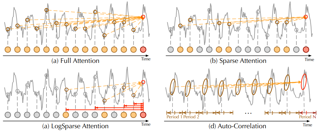 Figure 3: Auto-Correlation vs. self-attention family.
- Full Attention (a)는 모든 시간 지점 사이의 완전한 연결을 적응시킴
- Sparse Attention (b)은 제안된 유사도 지표를 기반으로 지점을 선택
- LogSparse Attention(c)은 지수적으로 증가하는 간격을 따라 지점을 선택
- Auto-Correlation (d)은 기본 주기 사이의 하위 시리즈 연결에 집중
4 Experiments
Datasets
Implementation details
Baselines
4.1 Main Results
4.2 Ablation studies
4.3 Model Analysis
5 Conclusion
- 실제 응용 프로그램에서 긴 시계열 예측 문제를 연구
- 그러나 복잡한 시간적 패턴으로 인해 모델이 신뢰할 수 있는 종속성을 학습하는 데 어려움
- Autoformer를 분해 아키텍처로 제안하여 시리즈 분해 블록을 내부 연산자로 포함시켜 중간 예측에서 장기 추세 부분을 점진적으로 집계
- 또한, 효율적인 Auto-Correlation 메커니즘을 설계하여 시리즈 수준에서 종속성 발견과 정보 집계를 수행
- 이는 이전의 self-attention family와 명확하게 다름
- Autoformer는 자연스럽게 $\mathcal{O}(L\log{L})$ 복잡도를 달성하고 넓은 범위의 실제 데이터셋에서 일관된 SOTA을 달성
Next: Autoformer(2)