간단한 classification

Breast Cancer Wisconsin (Diagnostic) Data Set

0. Settings

import numpy as np
import pandas as pd
import matplotlib.pyplot as plt
import seaborn as sns
import sklearn

file_name = '/kaggle/input/breast-cancer-wisconsin-data/data.csv'

df = pd.read_csv(
    file_name,
)

1. EDA

1.1. Preview

df.head()

	diagnosis	radius_mean	texture_mean	perimeter_mean	area_mean	smoothness_mean	compactness_mean	concavity_mean	concave points_mean	symmetry_mean	...	radius_worst	texture_worst	perimeter_worst	area_worst	smoothness_worst	compactness_worst	concavity_worst	concave points_worst	symmetry_worst	fractal_dimension_worst
0	1	17.99	10.38	122.80	1001.0	0.11840	0.27760	0.3001	0.14710	0.2419	...	25.38	17.33	184.60	2019.0	0.1622	0.6656	0.7119	0.2654	0.4601	0.11890
1	1	20.57	17.77	132.90	1326.0	0.08474	0.07864	0.0869	0.07017	0.1812	...	24.99	23.41	158.80	1956.0	0.1238	0.1866	0.2416	0.1860	0.2750	0.08902
2	1	19.69	21.25	130.00	1203.0	0.10960	0.15990	0.1974	0.12790	0.2069	...	23.57	25.53	152.50	1709.0	0.1444	0.4245	0.4504	0.2430	0.3613	0.08758
3	1	11.42	20.38	77.58	386.1	0.14250	0.28390	0.2414	0.10520	0.2597	...	14.91	26.50	98.87	567.7	0.2098	0.8663	0.6869	0.2575	0.6638	0.17300
4	1	20.29	14.34	135.10	1297.0	0.10030	0.13280	0.1980	0.10430	0.1809	...	22.54	16.67	152.20	1575.0	0.1374	0.2050	0.4000	0.1625	0.2364	0.07678

5 rows × 31 columns

df.info()

<class 'pandas.core.frame.DataFrame'>
RangeIndex: 569 entries, 0 to 568
Data columns (total 33 columns):
 #   Column                   Non-Null Count  Dtype  
---  ------                   --------------  -----  
 0   id                       569 non-null    int64  
 1   diagnosis                569 non-null    object 
 2   radius_mean              569 non-null    float64
 3   texture_mean             569 non-null    float64
 4   perimeter_mean           569 non-null    float64
 5   area_mean                569 non-null    float64
 6   smoothness_mean          569 non-null    float64
 7   compactness_mean         569 non-null    float64
 8   concavity_mean           569 non-null    float64
 9   concave points_mean      569 non-null    float64
 10  symmetry_mean            569 non-null    float64
 11  fractal_dimension_mean   569 non-null    float64
 12  radius_se                569 non-null    float64
 13  texture_se               569 non-null    float64
 14  perimeter_se             569 non-null    float64
 15  area_se                  569 non-null    float64
 16  smoothness_se            569 non-null    float64
 17  compactness_se           569 non-null    float64
 18  concavity_se             569 non-null    float64
 19  concave points_se        569 non-null    float64
 20  symmetry_se              569 non-null    float64
 21  fractal_dimension_se     569 non-null    float64
 22  radius_worst             569 non-null    float64
 23  texture_worst            569 non-null    float64
 24  perimeter_worst          569 non-null    float64
 25  area_worst               569 non-null    float64
 26  smoothness_worst         569 non-null    float64
 27  compactness_worst        569 non-null    float64
 28  concavity_worst          569 non-null    float64
 29  concave points_worst     569 non-null    float64
 30  symmetry_worst           569 non-null    float64
 31  fractal_dimension_worst  569 non-null    float64
 32  Unnamed: 32              0 non-null      float64
dtypes: float64(31), int64(1), object(1)
memory usage: 146.8+ KB

df.id.duplicated().sum()

0

# 중복된 id가 없으므로 id column을 제외하고 각 row를 독립적인 데이터로 사용
df = df.drop(['id'], axis=1)

1.1.1. 결측치 처리

# 마지막 컬럼 제외
df = df.iloc[:, :-1]

1.1.2. Label diagnosis

df.diagnosis.value_counts()

diagnosis
B    357
M    212
Name: count, dtype: int64

df['diagnosis'] = df['diagnosis'].apply(lambda x: 1 if x == 'M' else 0)
df.diagnosis.value_counts()

diagnosis
0    357
1    212
Name: count, dtype: int64

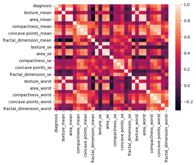
1.1.3. Correlations

corr = df.corr()

sns.heatmap(corr)
plt.show()

2. Predict

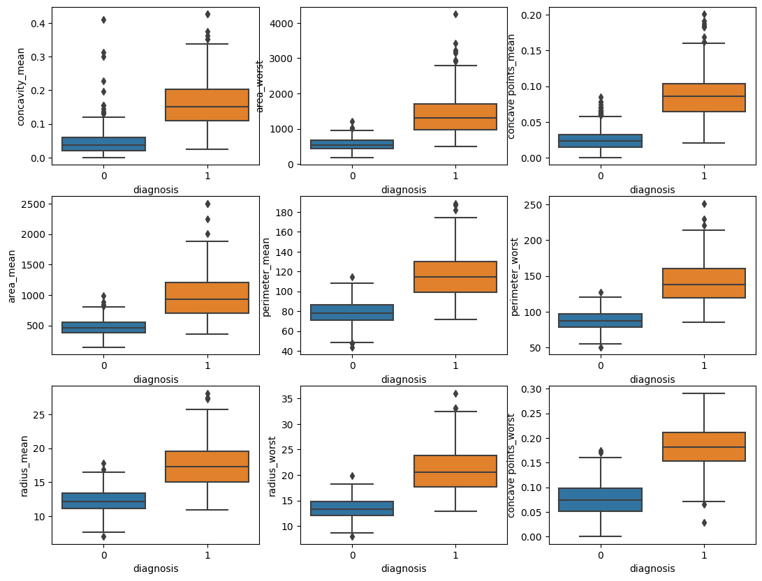
2.1. Data Selection

corr['diagnosis'].sort_values().tail(10)

concavity_mean          0.696360
area_mean               0.708984
radius_mean             0.730029
area_worst              0.733825
perimeter_mean          0.742636
radius_worst            0.776454
concave points_mean     0.776614
perimeter_worst         0.782914
concave points_worst    0.793566
diagnosis               1.000000
Name: diagnosis, dtype: float64

idx = corr['diagnosis'].sort_values().tail(10).index
X = df[idx].drop(['diagnosis'], axis=1)
y = df['diagnosis']

X.head()

	concavity_mean	area_mean	radius_mean	area_worst	perimeter_mean	radius_worst	concave points_mean	perimeter_worst	concave points_worst
0	0.3001	1001.0	17.99	2019.0	122.80	25.38	0.14710	184.60	0.2654
1	0.0869	1326.0	20.57	1956.0	132.90	24.99	0.07017	158.80	0.1860
2	0.1974	1203.0	19.69	1709.0	130.00	23.57	0.12790	152.50	0.2430
3	0.2414	386.1	11.42	567.7	77.58	14.91	0.10520	98.87	0.2575
4	0.1980	1297.0	20.29	1575.0	135.10	22.54	0.10430	152.20	0.1625

fig, axs = plt.subplots(nrows=3, ncols=3, figsize=(13, 10))

for i, col_name in enumerate(X.columns):
    sns.boxplot(y=X[col_name], x=y, ax=axs[i%3][i//3])
    
plt.show()

2.2. Machine Learning

from sklearn.preprocessing import StandardScaler, MinMaxScaler
from sklearn.neighbors import KNeighborsClassifier
from sklearn.pipeline import Pipeline
from sklearn.model_selection import GridSearchCV
from sklearn.model_selection import train_test_split

X_train, X_test, y_train, y_test = train_test_split(X, y, random_state=42)

pipe = Pipeline([
    ('scale', None),
    ('model', KNeighborsClassifier())
])

pipe.get_params()

{'memory': None,
 'steps': [('scale', None), ('model', KNeighborsClassifier())],
 'verbose': False,
 'scale': None,
 'model': KNeighborsClassifier(),
 'model__algorithm': 'auto',
 'model__leaf_size': 30,
 'model__metric': 'minkowski',
 'model__metric_params': None,
 'model__n_jobs': None,
 'model__n_neighbors': 5,
 'model__p': 2,
 'model__weights': 'uniform'}

param_grid = {
    'model__n_neighbors':[5,10],
    'scale': [StandardScaler(), MinMaxScaler()],
#     'model__class_weight': [{0:1, 1:v/2} for v in range(1,5)]
}



mod = GridSearchCV(
    estimator=pipe,
    param_grid=param_grid,
    cv=3
)

mod.fit(X_train, y_train)

pd.DataFrame(mod.cv_results_).T

	0	1	2	3
mean_fit_time	0.004918	0.004554	0.004715	0.004649
std_fit_time	0.000317	0.000055	0.000029	0.00001
mean_score_time	0.012827	0.012498	0.012517	0.012951
std_score_time	0.000298	0.000277	0.000072	0.000264
param_model__n_neighbors	5	5	10	10
param_scale	StandardScaler()	MinMaxScaler()	StandardScaler()	MinMaxScaler()
params	{'model__n_neighbors': 5, 'scale': StandardSca...	{'model__n_neighbors': 5, 'scale': MinMaxScale...	{'model__n_neighbors': 10, 'scale': StandardSc...	{'model__n_neighbors': 10, 'scale': MinMaxScal...
split0_test_score	0.943662	0.929577	0.93662	0.929577
split1_test_score	0.950704	0.93662	0.943662	0.943662
split2_test_score	0.93662	0.943662	0.93662	0.93662
mean_test_score	0.943662	0.93662	0.938967	0.93662
std_test_score	0.00575	0.00575	0.00332	0.00575
rank_test_score	1	3	2	3

mod.score(X_test, y_test)

0.951048951048951